The cover page

Main Technologies
I. Deep Learning
Deep learning generally refers to the classification and regression of unknown data by training multi-layer network structures, and simply speaking deep learning can be divided into two categories. One category is supervised learning methods, which include deep feedforward networks, convolutional neural networks, recurrent neural networks, etc. The other category is unsupervised learning methods, which include deep belief nets, deep Boltzmann machines, deep self-encoders, etc. Deep learning has a wide range of applications and can be widely used in image processing, speech recognition, natural language processing, etc.
In our robot, the main thing is to use deep learning to achieve object recognition, so we choose to use the very classic algorithm of the target detection Yolo series - Yolov3. it absorbs many points of the algorithm, while ensuring the speed, there is a certain accuracy, especially the recognition of small objects capability.

Figure. 1 yolov3 frame diagram
The three blue boxes in the figure above figure. 1 the three basic components of Yolov3.
CBL: the smallest component of the Yolov3 network structure, consisting of the triplet of Conv + Bn + Leaky_relu activation function.
Res unit: borrowing the residual structure from Resnet network, allowing the network to be built deeper
ResX: consists of a CBL and X residual components, which are the large components in Yolov3. The CBL in front of each Res module plays the role of downsampling, so after 5 Res modules, the feature map obtained is 608-> 304-> 152-> 76-> 38-> 19 in size.
Other basic operations
Concat: tensor stitching, will expand the dimension of two tensors, for example, 26 × 26 × 256 and 26 × 26 × 512 two tensor stitching, the result is 26 × 26 × 768. concat and cfg file in the router function is the same.
Add: tensor sum, tensor direct sum, will not expand the dimension, for example, 104 × 104 × 128 and 104 × 104 × 128 sum, the result is still 104 × 104 × 128. add and cfg file shortcut function the same.
Backbone
Inside the whole v3 structure, there is no pooling and fully connected layer. In the forward propagation process, the size transformation of the tensor is achieved by changing the step size of the convolution kernel, for example, stride=(2, 2), which is equivalent to reducing the image edge length by half (i.e., the area is reduced to 1/4 of the original size). In yolo_v2, going through 5 reductions will reduce the feature map to 1/25 of the original input size, i.e., 1/32. The input is 416x416, and the output is 13 × 13 (416/32 = 13).
darknet53frame diagram is shown in figure. 2
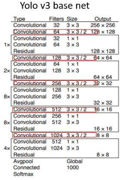
Figure. 2 darknet53frame diagram
Output
Yolov3 outputs a feature map with 3 different scales, as shown above for y1, y2, y3. This draws on FPN (feature pyramid networks), which uses multiple scales to detect targets of different sizes, the finer the grid cell the finer the object can be detected. y1, y2 and y3 have a depth of 255 and a regular edge length of 13:26:52. For the COCO category, there are 80 categories, so each box should output a probability for each category. yolov3 is set to predict 3 boxes per grid cell, so each box needs to have (x, y, w, h, confidence) five basic parameters, and then also have 80 categories of probabilities. So 3 × (5 + 80) = 255.
II, the chassis-related technical description
(1) Overall control logic is shown in figure. 3
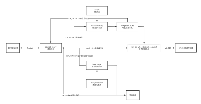
Figure. 3 overall logic diagram
(2) SLAM map building
Self-built maps are built using the SLAM building algorithm. Using this algorithm, the robot is manually manipulated by humans to build the map. The map building process is based on sensors to obtain a map of the current local environment, and to integrate the local map into the global map, in which a coordinate transformation, which includes translation and rotation, is performed to the location of the global map. When the local map is initialized, the pixel value 128 is used to indicate that the current raster is uncertain (the range of pixel values used is 0-255), then, if the current raster is an obstacle, we set it to 0, otherwise, it is 255. let the value of the raster on the global raster map is distributed in 0-255, the smaller the value corresponding to the raster is less than 128, the greater the probability that it is an obstacle, the larger the value corresponding to the raster is greater than 128, the greater the probability of the obstacle.
Fusion map filtering using Bayes

Z: Value observations (each observation is derived from a local map with only two states: occupied, idle)
P(statei∣Zt ): the probability that grid i is occupied by an obstacle after fusing the observations at moment t+1
P(statei∣Zt): the probability that grid i is occupied by an obstacle after fusing the observations at time t, i.e., the probability of the last observation
P0(statei∣Zt+1): the probability that grid i is occupied by an obstacle judged solely from the observation at moment t+1, i.e., the prediction probability can generally be taken as a constant, such as P0(statei∣Zt=occupied)=0.6, P0(statei∣Zt=vacant)=0.3
(3) Navigation robot autonomous obstacle avoidance navigation
The navigation function package is shown in the figure. 4. The most central node is move_base, which is the final actuator for the motion control of the navigation process. move_base subscribes to the user-published navigation target move_base_simple/goal and sends the real-time motion control signal cmd_vel down to the chassis to achieve the final motion control. The various navigation algorithm modules in move_base are called in the form of plug-ins, so that different algorithms can be easily replaced to suit different applications, including global_planner for global path planning, local_planner for local path planning, golobal_costmap for global cost map to describe the global environment information, local_costmap for local_costmap is used to describe the local environment information, and recovery_behaviors is a recovery policy used for automatic escape recovery after the robot encounters an obstacle. Then comes the amcl node, which uses particle filtering algorithm to achieve global localization of the robot and provides global location information for robot navigation. Then there is the map_server node, which provides the environment map information for navigation by calling the map obtained from the previous SLAM build. The last is to provide the tf information, odometry odom information, and LiDAR information scan related to the robot model.
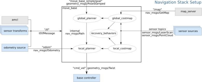
Figure. 4 Navigation node diagram
Path planning: The core of robot navigation is path planning. Path planning is to find a way to reach the target with low cost by using environmental obstacle information. There are two types of path planning used in navigation, namely global_planner and local_planner. global_planner is more of a strategic strategy that takes the global picture into account and plans a path that is as short and easy to execute as possible. Under the guidance of the global path, the robot also needs to consider the surrounding real-time obstacles and develop an avoidance strategy when walking, which is what the local path planning has to accomplish.
(4) Speech recognition
Use Iflytek voice function to realize voice interaction function. The Iflytek open platform is used to implement the voice output function of ROS. The task flow diagram is as figure. 5 and figure. 6. In the terminal, a string is posted to the /voiceWords topic through the terminal to enable the text-to-speech function. Subsequently, the text-to-speech function is implemented by modifying tts_subscribe.cpp, and the converted speech is broadcasted in real time.

Figure. 5 Schematic diagram of text-to-speech
After that, to implement ros simultaneous input and output of speech, firstly, in the terminal, post wakeup words to the /voiceWakeup topic and turn on the speech to text function. Then, turn on the text-to-speech function to get the text from the /voiceWords topic and play it back as speech.

Figure. 6 Text-to-speech schematic diagram of the topic to obtain the text-to-speech schematic diagram
(5) Socket communication
Sockets ensure communication between different computers, that is, network communication. For websites, the communication model is between a server and a client. A socket object is created at both ends, and then data is transferred through the socket object. Usually the server is in an infinite loop, waiting for a connection from the client.
Basic steps for socket communication.
Server side.
Step 1: Create a Socket pair for listening to connections.
Step 2: Create an EndPoint pair with the specified port number and the server's ip.
Step 3: Bind the EndPoint with the Bind() method of the socket object.
Step 4: start listening with the Listen() method of the socket object.
Step 5: Receive the connection from the client and create a new socket object for communication with the client using the Accept() method of the socket object;
Step 6: Always remember to close the socket after the communication is finished;
Client side:
Step 1: Create a socket pair.
Step 2: Create an EndPoint pair with the specified port number and the server's ip.
Step 3: send a connection request to the server using the Connect() method of the socket object with the EndPoint object created above as a parameter.
Step 4: if the connection is successful, send a message to the server using the Send() method of the socket object.
Step 5: Receive the message from the server using the Receive() method of the socket object;
Step 6: always remember to close the socket when the communication is finished.
socket Communication diagram is shown in figure. 7
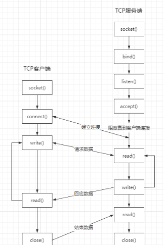
Figure. 7 socket Communication diagram
Media materials
This part contains certain some vivid photos and interseting videos.
Figures 8, 9, 10 and 11 respectively show the appearance of the service robot.

Figures. 8 side view of the service robot
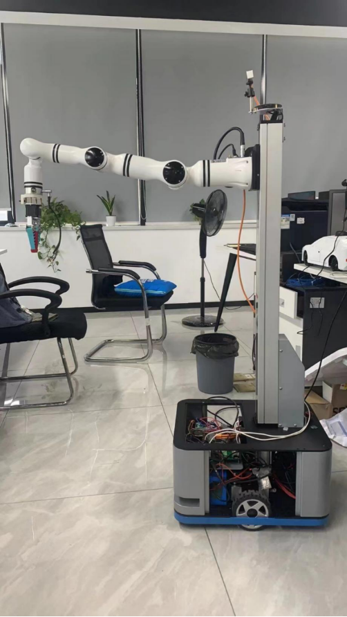
Figures. 9 side view of the service robot

Figures. 10 direct top view of the service robot

Figures. 11 rear view of the service robot
Figures 11 and 12 respectively show the 3d drawings of the service robot.
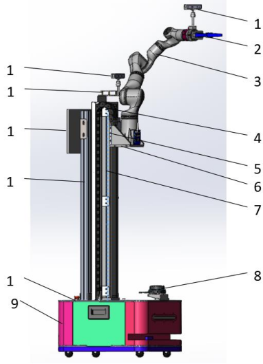
Figures. 12 General diagram of indoor service robot
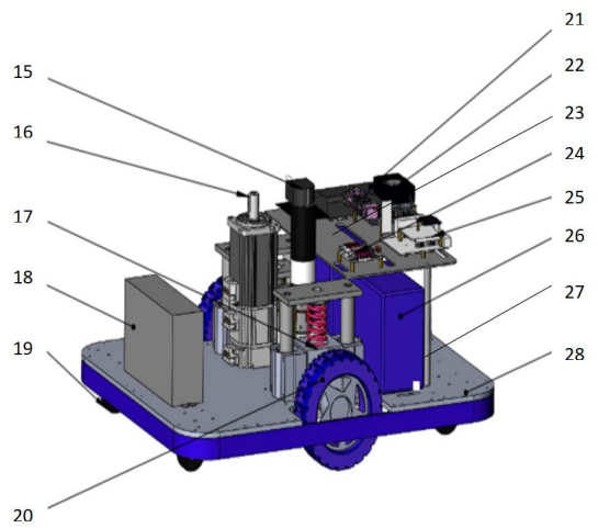
Figures. 13 Interior model diagram of indoor service robot chassis
The following links are related to some interesting videos, due to copyright issues can only be presented in the form of links.
https://www.youtube.com/watch?v=UHYlQjFlfak
https://www.youtube.com/watch?v=_filGYIdsig
https://www.youtube.com/watch?v=saVZtgPyyJQ
https://www.youtube.com/watch?v=Uz_i_sjVhIM
https://www.youtube.com/watch?v=AH_eQS5Tzyo


